
Radial functions: an experiment against Hartree–Fock
Question. The app draws and integrates valence orbitals with two different radial functions: Slater's single exponents in the orbital layer (π overlaps, Löwdin densities, the π maps) and effective-charge hydrogenic functions in the 3D viewer. Which one is closer to a real atomic orbital, and does the difference matter for what the app shows?
Forecast. Written down before any number was computed: FORECAST.md (10 Oct 2026, 10:45).
The reference, and how it was checked
There are no published orbitals I could download here, so I computed them: Hartree–Fock for each free atom (atomic_hf.py), using Slater's average-of-configuration energy (1960) in a large even-tempered Gaussian basis (21–40 functions per angular momentum).
- Closed shells (Be, Ne, Mg, Ar, Kr, Xe) reproduce the numerical Hartree–Fock limit to 2 × 10⁻⁶ – 4 × 10⁻⁴ hartree. The Ne 2p ⟨r⟩ comes out at 0.965 bohr, the tabulated value.
- Open shells: from the same orbitals, the ground-term energy (³P, ⁴S or ²P) lands 0.01–1.6 mEh above the published Hartree–Fock limit, never below, as it must for orbitals not optimised for that term:
| Atom | frozen-orbital term energy | Hartree–Fock limit | difference (mEh) |
|---|---|---|---|
| C | -37.68834 | -37.68862 | +0.28 |
| N | -54.39933 | -54.40093 | +1.60 |
| O | -74.80926 | -74.80940 | +0.14 |
| F | -99.40934 | -99.40935 | +0.01 |
| P | -340.71782 | -340.71878 | +0.96 |
| S | -397.50478 | -397.50490 | +0.12 |
| Cl | -459.48202 | -459.48207 | +0.05 |
| Br | -2572.44113 | -2572.44133 | +0.21 |
| I | -6917.98020 | -6917.98089 | +0.69 |
A first attempt with fractionally occupied open shells failed this check by 150–550 mEh: it lets an electron repel itself, which swells the open shell (carbon 2p ⟨r⟩ came out 23 % too large). Those numbers were discarded. That failure is why the check is in the script.
Results
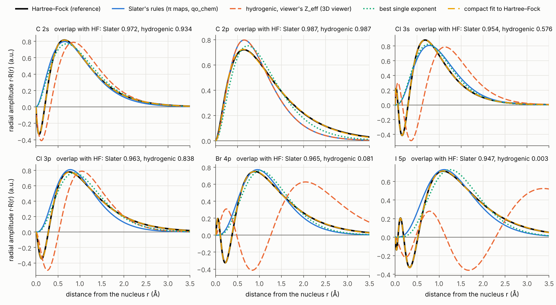
1 · The atomic functions. Overlap with Hartree–Fock (1 = identical), and in brackets the error in ⟨r⟩:
| Orbital | HF ⟨r⟩ (Å) | Slater | hydrogenic (viewer) | best single ζ | compact fit |
|---|---|---|---|---|---|
| C 2s | 0.839 | 0.972 (-3 %) | 0.934 (+16 %) | 0.975 (+4 %) | 1.000 (+0 %) |
| C 2p | 0.922 | 0.987 (-12 %) | 0.987 (-12 %) | 0.994 (-1 %) | 1.000 (-0 %) |
| N 2s | 0.702 | 0.970 (-3 %) | 0.936 (+16 %) | 0.974 (+4 %) | 1.000 (+0 %) |
| N 2p | 0.766 | 0.986 (-11 %) | 0.986 (-11 %) | 0.992 (-1 %) | 1.000 (-0 %) |
| O 2s | 0.604 | 0.968 (-4 %) | 0.938 (+16 %) | 0.973 (+4 %) | 1.000 (+0 %) |
| O 2p | 0.656 | 0.985 (-11 %) | 0.985 (-11 %) | 0.991 (-1 %) | 1.000 (-0 %) |
| F 2s | 0.530 | 0.967 (-4 %) | 0.940 (+15 %) | 0.972 (+5 %) | 1.000 (-0 %) |
| F 2p | 0.574 | 0.984 (-11 %) | 0.984 (-11 %) | 0.990 (-1 %) | 1.000 (-0 %) |
| P 3s | 1.020 | 0.958 (+13 %) | 0.533 (+46 %) | 0.963 (+6 %) | 1.000 (-0 %) |
| P 3p | 1.254 | 0.968 (-8 %) | 0.833 (+10 %) | 0.978 (+3 %) | 1.000 (+0 %) |
| S 3s | 0.910 | 0.956 (+12 %) | 0.555 (+44 %) | 0.959 (+6 %) | 1.000 (-0 %) |
| S 3p | 1.095 | 0.966 (-7 %) | 0.835 (+11 %) | 0.975 (+3 %) | 1.000 (+0 %) |
| Cl 3s | 0.823 | 0.954 (+11 %) | 0.576 (+42 %) | 0.955 (+7 %) | 1.000 (-0 %) |
| Cl 3p | 0.975 | 0.963 (-7 %) | 0.838 (+11 %) | 0.972 (+4 %) | 1.000 (+0 %) |
| Br 4s | 0.920 | 0.945 (+18 %) | -0.119 (+126 %) | 0.959 (+6 %) | 1.000 (+0 %) |
| Br 4p | 1.117 | 0.965 (-3 %) | 0.081 (+79 %) | 0.970 (+3 %) | 1.000 (-0 %) |
| I 5s | 1.108 | 0.940 (+13 %) | 0.061 (+194 %) | 0.953 (+6 %) | 1.000 (+0 %) |
| I 5p | 1.324 | 0.947 (-5 %) | 0.003 (+139 %) | 0.964 (+4 %) | 1.000 (-0 %) |
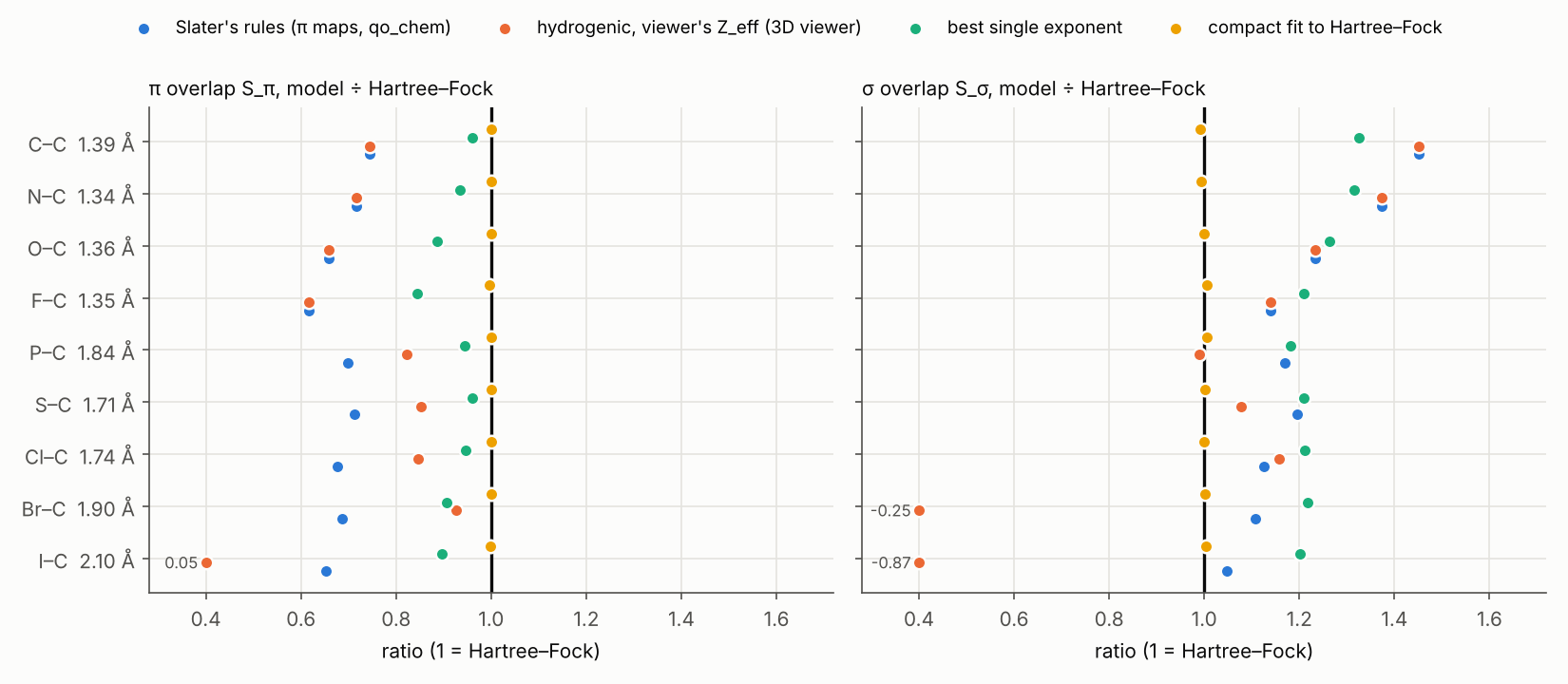
2 · What the orbital layer integrates. Two-centre overlaps of p orbitals with a carbon 2p at typical bond lengths, as a ratio to the Hartree–Fock value (both atoms described by the same model):
| Bond | R (Å) | HF S_π | Slater | hydrogenic | best single ζ | compact fit | HF S_σ | Slater | hydrogenic | best single ζ | compact fit |
|---|---|---|---|---|---|---|---|---|---|---|---|
| C–C | 1.39 | 0.333 | 0.74 | 0.74 | 0.96 | 1.00 | 0.228 | 1.45 | 1.45 | 1.33 | 0.99 |
| N–C | 1.34 | 0.299 | 0.72 | 0.72 | 0.94 | 1.00 | 0.236 | 1.37 | 1.37 | 1.32 | 0.99 |
| O–C | 1.36 | 0.245 | 0.66 | 0.66 | 0.89 | 1.00 | 0.241 | 1.23 | 1.23 | 1.26 | 1.00 |
| F–C | 1.35 | 0.210 | 0.62 | 0.62 | 0.85 | 1.00 | 0.231 | 1.14 | 1.14 | 1.21 | 1.01 |
| P–C | 1.84 | 0.251 | 0.70 | 0.82 | 0.94 | 1.00 | 0.282 | 1.17 | 0.99 | 1.18 | 1.01 |
| S–C | 1.71 | 0.257 | 0.71 | 0.85 | 0.96 | 1.00 | 0.289 | 1.19 | 1.08 | 1.21 | 1.00 |
| Cl–C | 1.74 | 0.216 | 0.68 | 0.85 | 0.95 | 1.00 | 0.294 | 1.12 | 1.16 | 1.21 | 1.00 |
| Br–C | 1.90 | 0.203 | 0.69 | 0.93 | 0.91 | 1.00 | 0.300 | 1.11 | -0.25 | 1.22 | 1.00 |
| I–C | 2.10 | 0.190 | 0.65 | 0.05 | 0.90 | 1.00 | 0.298 | 1.05 | -0.87 | 1.20 | 1.00 |
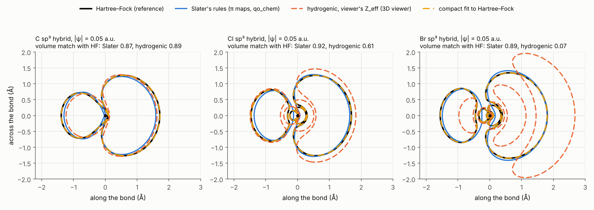
3 · What the viewer draws. sp^λ hybrids, isosurface at |ψ| = 0.05 a.u.: the fraction of the Hartree–Fock lobe volume that each model reproduces (intersection over union, positive / negative lobe):
| Hybrid | Slater | hydrogenic (viewer) | best single ζ | compact fit | HF: \|ψ(nucleus)\| ÷ lobe max |
|---|---|---|---|---|---|
| C sp³ | 0.87 / 0.83 | 0.89 / 0.71 | 0.96 / 0.85 | 1.00 / 0.99 | 1.8 |
| O–H in water, sp^3.99 | 0.81 / 0.76 | 0.84 / 0.64 | 0.93 / 0.88 | 0.99 / 0.99 | 1.5 |
| N sp² | 0.85 / 0.80 | 0.87 / 0.64 | 0.95 / 0.85 | 0.99 / 0.98 | 2.0 |
| Cl sp³ | 0.92 / 0.78 | 0.61 / 0.71 | 0.90 / 0.86 | 1.00 / 0.99 | 4.3 |
| Br sp³ | 0.89 / 0.79 | 0.07 / 0.00 | 0.91 / 0.78 | 1.00 / 0.99 | 5.7 |
| I sp³ | 0.90 / 0.70 | 0.09 / 0.05 | 0.88 / 0.68 | 1.00 / 0.99 | 7.3 |
Forecast against outcome
| Forecast | Outcome | ||
|---|---|---|---|
| F1 | 2p: Slater = hydrogenic; ⟨r⟩ 5–10 % too small; overlap ≥ 0.98 | identical; ⟨r⟩ 11–12 % too small; overlap 0.984–0.987 | size of the error underestimated |
| F2 | HF 2s node ≈ 0.1 Å; Slater's 2s beats the hydrogenic 2s | node at 0.13–0.20 Å; Slater 0.97 vs hydrogenic 0.93–0.94 | right, node position off by up to 2× |
| F3 | 3s/3p: both ≈ 0.95–0.97; S_π(C–Cl) from Slater 10–20 % low | Slater 0.95–0.97; hydrogenic 3p 0.83–0.84, 3s 0.53–0.58; S_π 32 % low | wrong: hydrogenic far worse, Slater's overlap error larger |
| F4 | viewer's Br/I ⟨r⟩ +60 %, overlap < 0.9; Slater ~10 % too compact | ⟨r⟩ +79 % and +139 %, overlap 0.08 and 0.003; Slater only 3–5 % too compact | wrong in size: the viewer's Br and I are different orbitals altogether |
| F5 | best single ζ ≥ 0.99 for 2p; compact fit ≥ 0.999 everywhere | 0.990–0.994; ≥ 0.99992 | right |
| F6 | S_π(C–C) larger with HF (≈ 0.27) than Slater's 0.248 | 0.333: Slater 26 % low | direction right, size wrong |
| — | (not forecast) | S_σ goes the other way: Slater overestimates it by 5–45 %, and with HF orbitals S_π > S_σ for C–C at 1.39 Å | the diffuse HF lobes reach past each other, so σ overlap is already past its maximum |
What it means for the app
- Not affected: Hückel energies, charges, bond orders and the three pKa descriptors (Q_site, V_probe, ΔE_deloc). They never use a radial function.
- Affected, orbital layer: the overlap matrix S and the Löwdin matrix M = S^-1/2 behind the π density, interference and orbital maps. Slater's 2p is 11–12 % too compact and the π overlaps are 26–38 % too small. How much that changes the maps themselves I have not measured yet.
- Affected, 3D viewer: for Br and I the viewer uses Z_eff = 6.10, copied from chlorine, with n = 4 and 5. The result has essentially nothing in common with the real 4p and 5p (overlap 0.08 and 0.003). That is a bug. For P, S and Cl the hydrogenic 3s puts its nodes in the wrong place (overlap 0.53–0.58).
- Affected, the viewer's isovalue rule: the viewer draws each surface at a fraction of max |ψ| on its grid, and the grid includes the nucleus. A realistic s function is largest at the nucleus: in a Hartree–Fock hybrid, |ψ| at the nucleus is 1.5–7.3 times the lobe maximum. Feed it realistic orbitals with the present rule and the nucleus would set the isovalue, shrinking the lobes. An absolute isovalue (|ψ| = 0.05 a.u., the usual choice in quantum chemistry) avoids that.
Recommendation
Use one radial table for both the orbital layer and the viewer: the compact fits (2–6 Slater terms per orbital, overlap with Hartree–Fock ≥ 0.99992; parameters in results.json under compact_terms).
- The orbital layer keeps its quadrature: an overlap of two sums is the sum of the pairwise Slater overlaps it already computes.
- The viewer evaluates Σ c_k r^(N_k−1) e^(−ζ_k r) instead of one Laguerre polynomial: a few exponentials per grid point.
- At the same time, switch the viewer to an absolute isovalue.
The idea is old. Clementi and Raimondi (1963) refitted single exponents to Hartree–Fock atoms; Clementi and Roetti (1974) tabulated Hartree–Fock orbitals as short Slater sums. This experiment redoes it for the elements the app uses and measures what it changes on screen.
Limits of this experiment
- The reference is the free atom. Orbitals contract somewhat in molecules; minimal basis sets optimised on molecules go the other way from these fits (Hehre, Stewart and Pople 1969 used ζ = 1.72 for carbon, more compact than Slater's 1.625). Free-atom Hartree–Fock is a clean, reproducible definition of an atomic orbital, not the last word on orbitals inside a molecule.
- Average-of-configuration orbitals, not term-specific ones (differences of order 1 % in ⟨r⟩).
- Non-relativistic: for iodine the 5p is slightly affected by relativity (spin–orbit splitting is ignored).
What happened next
Version 16.1 adopted the recommendation. make_radial_table.py fits the valence ns and np orbitals of 16 elements (H, B, C, N, O, F, Na, Mg, Si, P, S, Cl, K, Ca, Br, I; every overlap with Hartree–Fock ≥ 0.9999) into qo_chem/data/radial_fits.json. The orbital layer's overlaps, the π maps and the 3D viewer's surfaces now read that one table, and the viewer draws every surface at a fixed |ψ| in atomic units. The hydrogenic functions, including the wrong bromine and iodine charges, are gone. The pKa descriptors did not move, as predicted: they never used a radial function.
Reproduce
python tools/radial/atomic_hf.py          # validation against the Hartree–Fock limit
python tools/radial/radial_benchmark.py   # about 2½ minutes on one core: results.json, curves.npz
python tools/radial/plot_results.py       # the three figures
python tools/radial/make_radial_table.py  # the table the app uses (about 3 minutes)